Predictive Uncertainty with Neural Networks for the GammaTPC Telescope Concept

Uncertainty in Physics

Experimental physicists spend most of their research time doing 2 things: building their experiment, and trying to figure out how wrong their results could be. You’ll notice that I skipped right over the part where you actually do your experiment and analyze your data. It’s not that those things don’t happen, it’s just that trying to figure out what you don’t know or didn’t account for is usually a lot harder than doing the thing you set out to do! After all, a result or measurement doesn’t mean much if you don’t know how wrong it could be.

The Muon G-2 experiment is located at Fermilab National Accelerator Laboratory in Batavia, Illinois. This image shows the muon storage ring that is the primary component of the experiment. You can see that it's pretty big. This image is taken from their website.

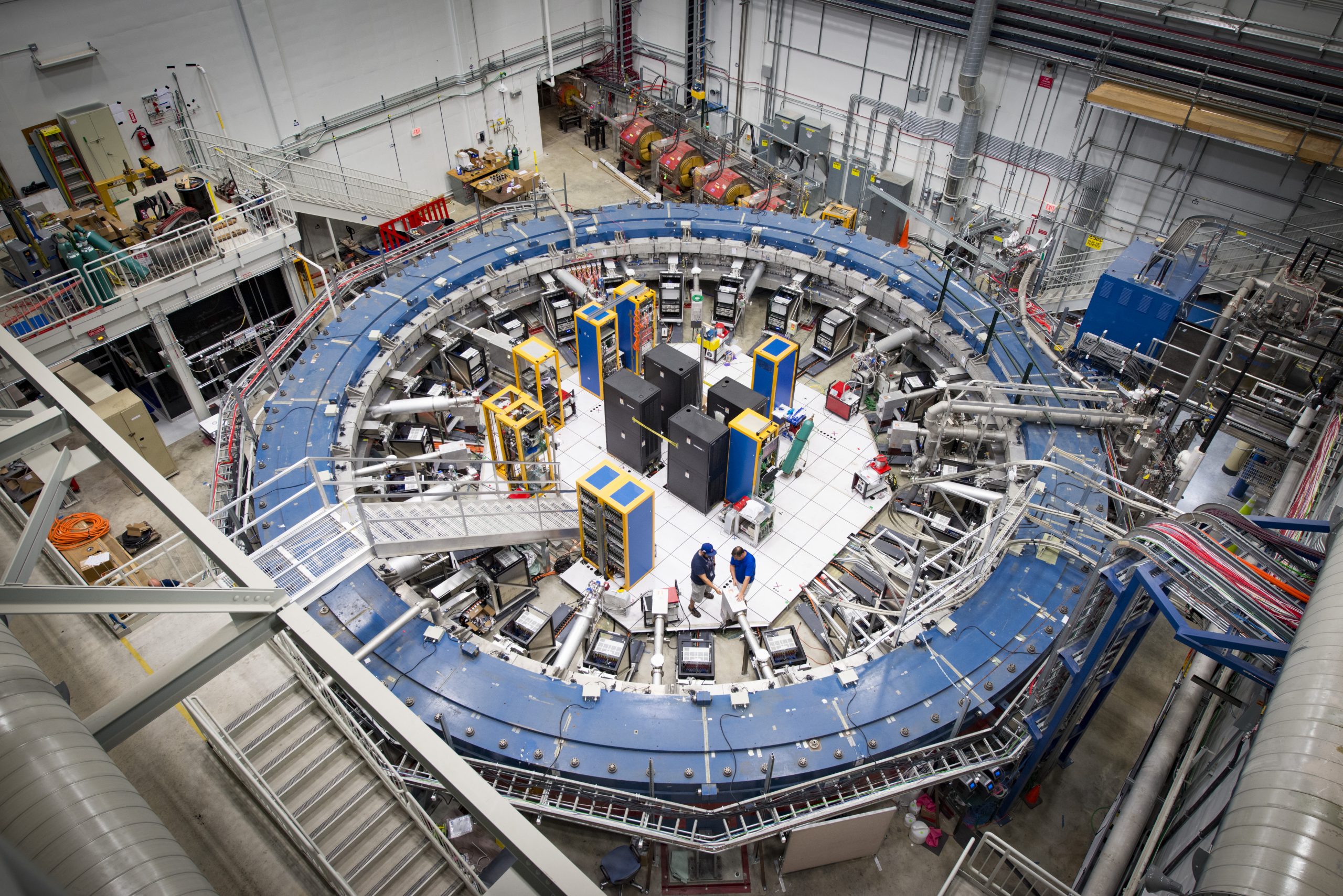
Take the case of the Muon g-2 experiment at Fermilab. This experiment was built make an extreeeemely precise measurement of something called the “anomalous magentic moment” of the muon¹. The reason physicists are interested in measuring this thing? In large part, it’s because the value that is predicted by particle theory does not agree with the number that has been measured with experiments. But it’s not just the fact that the numbers are different that is interesting, it’s the fact that experimentalists have been able to measure this number to incredible precision, and it’s waaay off from what theorists and their integrals say it should be. Uncertainty estimation (in this case, very small uncertainty estimation), is the linchpin of this experiment.

Physicists are also very excited to use machine learning in their research. However, most machine learning algorithms do not include any way to estimate the uncertainty of their predictions. This is a huge problem for physicists if they want to use the output of a machine learning model to infer anything interesting. To be sure, there are use cases in physics for machine learning with no uncertainty estimation, but you probably can’t unlock the full potential of machine learning models if you have to constrain the use of them to the parts of an analysis where uncertainty quantification is not necessary.

Uncertainty in Machine Learning

Self-driving cars are only as safe as their algorithms. This image is taken from this electrek article.

A lack of uncertainty quantification in machine learning is also a huge problem for other people, with an obvious example being the people who are trying to create self-driving cars. If your car pulls up to an intersection and thinks there’s no stop sign, should it still stop? How sure is it that there’s no stop sign? Is it worse for a car to accidentally stop at an intersection where there is not actually a stop sign, or to blow through a stop sign at an intersection where there could be pedestrians expecting it to stop? If the decision-making algorithm the car is using can only say “there is a stop sign” or “there is not a stop sign”, then it’s always going to treat those two possible mistakes as equally bad, even though the car speeding though a stop sign is clearly much worse than stopping (or at least slowing down) at an intersection with no stop sign. Ideally you want the car to say to itself “I can’t really tell if there’s a stop sign here, so I’ll slow down and keep looking until I can get a better idea”. You may recognize this as what probably goes through your head in this situation as well. We’re all doing uncertainty quantification all the time!

Being such an important topic, it’s unsurprising that Uncertainty Quantification (UQ) is a hot topic these days in machine learning research. There are a bunch of different approaches to quantify predictive uncertainty in your machine learning model, but I’m going to describe one that I have used in the past, and that I think is elegant and seems to work quite well! The rest of the sections in this post require some understanding of Bayesian statistics, so if you are not familiar with those words, or what a prior or posterior distribution are, check out this other post I wrote.

Flavors of Uncertainty

When physicists quantify their uncertainties, they usually break them up into two components: statistical and systematic. Statistical uncertainty refers to the fact that, because you only get to do one experiment to measure something (or at least a fixed number of them), you aren’t going to get the exact true value of the parameter you are trying to measure from your data. There’s a canonical example where you are trying to estimate the average height of a group of people by measuring their heights one at a time. Your best guess is going to be the average of the heights you have measured (assuming you are randomly sampling from the population of people), but the average height of the few people you’ve actually measured isn’t going to be the exact same as the average height of the whole group. Statistical uncertainty represents that difference. Systematic uncertainty is sort of a catch-all for all other types of possible sources of error, like: is the ruler you are using to measure people accurate? does the set of people you have measured have any systematic differences with the full population (i.e. you aren’t sampling truly randomly)? could the average height of the population be changing over time (e.g. lots of babies born)?

Thomas Bayes would like you to quantify your knowledge please. This image is from his Wikipedia page.

In Machine Learning, uncertainty is also broken up into two components that are in many ways similar to the way it is done in physics. They are: aleatoric and epistemic. Aleatoric uncertainty is essentially a measure of the variance of your data. If the population whose average height you are trying to measure comes from all ages, that group will likely have a high level of aleatoric uncertainty, while if they are all the same age and sex, the aleatoric uncertainty will probably be lower. Epistemic uncertainty refers to uncertainty in the model itself, i.e. how confident a model is in its own predictions. Estimating the average height of a population does not require a complex model, but if you are trying to do something more complicated, like classifying pictures of animals by species, you will probably need a much more complex model that will have some degree of uncertainty when it makes predictions. In many situations, as described above, having access to this source of uncertainty can be very useful.

GammaTPC and Evidential Deep Learning

I’ve been working on a project to design a space-based telescope to look for gamma-rays of a particular type that have been a bit neglected for the last few decades. This telescope will contain a bunch of liquid argon, where the gamma-rays will scatter off of electrons in the argon. When they scatter, the hit electron starts flying through the argon, leaving behind a trail of destruction (i.e. other ionized electrons) before it eventually runs out of energy and stops. If we can precisely measure the initial locations of several scatters, we can use physics and math to reconstruct where the gamma-ray must have come from. Because these scattered electrons are leaving a cloud/track of ionized electrons behind, we need to be able to determine where the beginning of the track is to successfully make this measurement. This telescope will be able to produce a 3D-grid reconstruction of the electron track, so it’s plausible that a 3D convolutional neural network will be able to do a good job in reconstructing the location of the initial scatter.

Left: A gamma-ray will scatter multiple times in the detector, and if you can figure out the order and locations, you can tell which direction it came from. Right: An example electron track (line), and the pixelated readout that the detector actually sees (circles). The circles are sized proportionally to the amount of charge measured at that location.

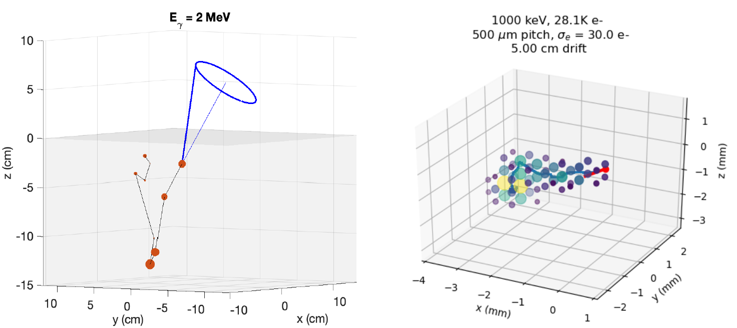
Precisely measuring the position of these electron scatters is key, but obtaining an uncertainty estimate for the observations is also very useful. If we know that a particular electron scatter is poorly measured, for whatever reason, it can be better to just completely ignore that data point, rather than include it in our data set knowing that it may be throwing off our measurements. I and several collaborators at SLAC have a paper out where we did just that. You can also find Jupyter notebooks to recreate the analysis here. We tested several different kinds of uncertainty estimating models on our problem, and determined that an approach from 2020, called Evidential Deep Learning, worked the best for us. Evidential Deep Learning works well because it makes use of the handy mathematical relationships between conjugate distributions that I discuss in another post to give you an uncertainty estimate without having to run the model a bunch of times (like an ensemble-based approach), or use a Bayesian neural network which can be much more computationally expensive. We also found that it performed better than other options in some key statistical metrics.

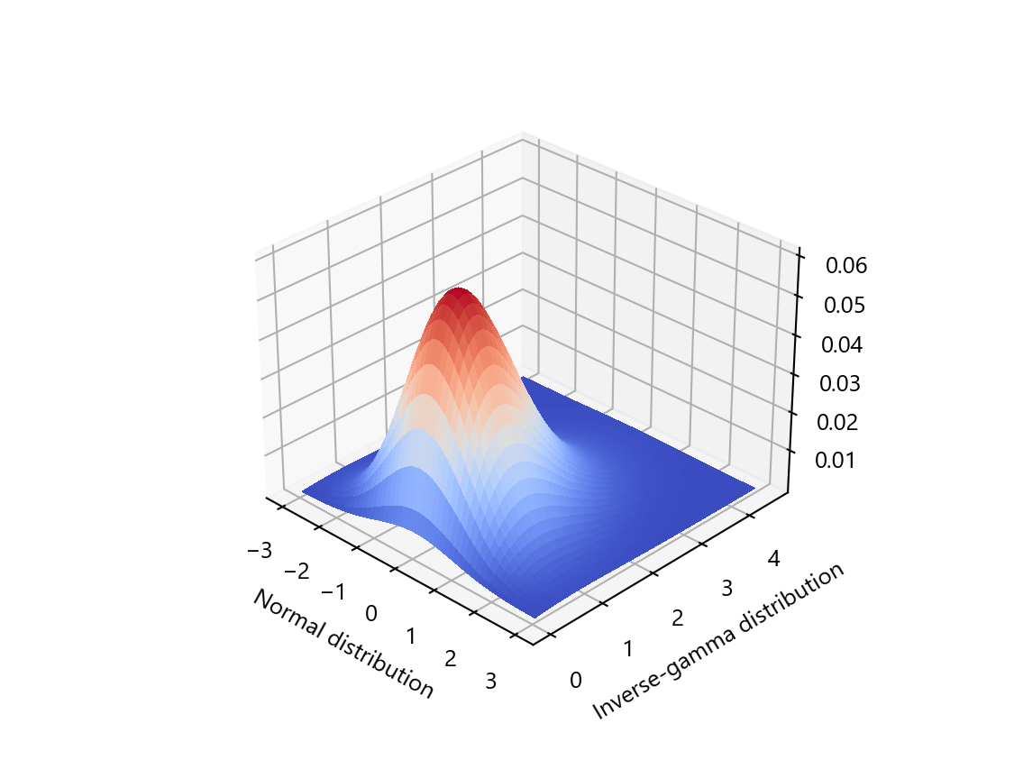
We are trying to predict the location of an electron scatter from a 3D grid showing the track that it left as it traveled through its argon medium. Minimally, this requires a model that produces 3 real numbers as output: predictions for the x, y, and z components of the location. These can be compared to the true simulated locations, and if the loss function (i.e. likelihood) being used is the mean-squared-error, that comparison should follow a normal distribution. In Evidential Deep Learning, we no longer try to just predict 3 numbers, but instead we actually try to predict 12 numbers, 4 for each cardinal direction prediction. These numbers are the parameters characterizing a normal-inverse-gamma distribution, which is the cojugate prior for a normal likelihood with an unknown mean and unknown variance (i.e. our likelihood). In this case, the normal likelihood in some sense represents the distribution of our data set, with the mean being predictions for the electron track head locations, and the variance being the aleatoric uncertainty. The normal-inverse-gamma posterior then is effectively the epistemic uncertainty the model has for both its predictions and its estimate of the aleatoric uncertainty. When we train our model to predict all of the parameters for the posterior distribution (called hyperparameters), we are essentially training it to estimate a range of plausible predictions for each electron track, rather than just a single point estimate. After the model is trained, we can feed in new examples of electron tracks, and then use the predicted normal-inverse-gamma hyperparameters to get a prediction interval.

A normal-inverse-gamma distribution is a joint probability distribution, which is the product of two unidimensional distributions. It has 2 random variables, and so its density function is 2D.

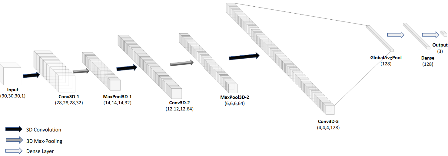
To find the heads of the electron tracks, we designed a multi-layer 3D convolutional neural network with 3 convolutional layers, 2 max pooling layers, and 1 global average pooling layer, followed by a feed-forward layer producing the final predictions. The model shown in the figure below is for a deterministic model we created as a benchmark to measure the Evidential model against. You can tell this because it ends with a length 3 vector for predicting the $X$, $Y$, and $Z$ components of the location. A very handy feature of Evidential Deep Learning is that it only requires swapping out the final layer for one that predicts 4x the number of outputs, and then altering the loss function appropriately. Furthermore, the author of the original paper has written a Python package that has code that can essentially be dropped into your existing setup. Instead of using the mean-squared-error for a loss function, you use the negative-log-likelihood (NLL) of the normal-inverse-gamma distribution, since minimizing the NLL produces the same optimized parameters as maximizing the likelihood does. And maximizing the likelihood while training your neural network essentially means that you are maximizing the ability of your network to predict the correct outputs from a given set of inputs.

We use convolutional layers for finding the track head because they have locality (i.e. they are aware of the physical layout of the pixels). Combining them with the pooling layers also makes the network essentially translation invariant, which we want because in principle the track head can be anywhere in the image.

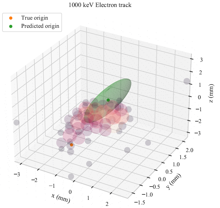
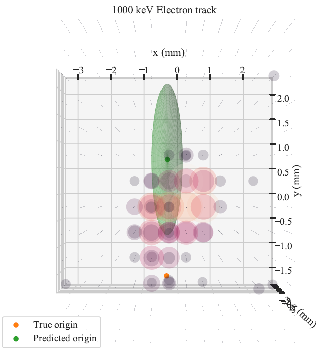
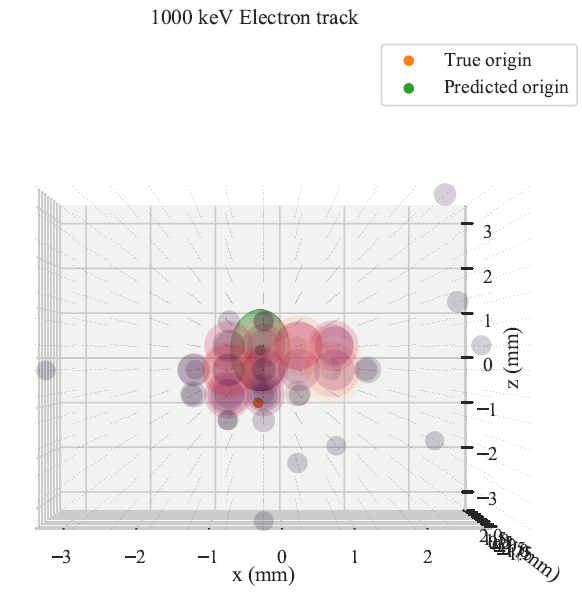
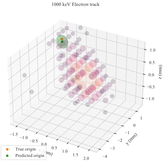
Once we train our network, we can use it to predict track head locations for samples in our validation dataset. We get predictions that look like what you see in the figure below. You can see the readout of each pixel given by the circles, which scale in both size and color with the amount of charge measured at that location. The predicted track head location is given by the green ellipsoid. You can see that when the prediction is off, the ellipsoid tends to be bigger, indicating that the network is less certain of its prediction. You may notice that the ellipsoids are all aligned with the cardinal axes, even though the actual error in general is not. This is because we have made predictions for the $X$, $Y$, and $Z$ components for the track head independently, so the uncertainty estimates are also independent. To move beyond this, we need to allow for correlated predictions and errors. This should also make the network more accurate, and “only” requires changing the posterior from a normal-inverse-gamma distribution to a multivariate-normal-inverse-Wishart, which is a higher dimensional generalization of the normal-inverse-gamma distribution. This is a project for another day though!

The uncertainty estimate (green ellipsoid) tends to be larger when the error is larger in each dimension. These are 3 views of the same event.

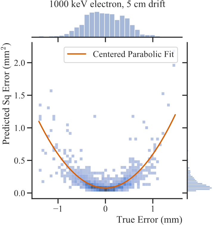
The below figure shows the predicted squared error against the true error for the validation dataset. If the network were estimating its errors perfectly, this data would follow the simplest parabola $\sigma^2_p = \epsilon_t^2$. The fit here is a little too wide, but the general trend is accurate, meaning that the network is successfully estimating its epistemic uncertainty, albeit undershooting it in general.

This histogram is fitted to a parabola with no linear component.

If you want to see more details of this analysis, check out the paper, published soon in the Astrophysical Journal (I hope!).

1. A muon is a fundamental particle sort of like a heavier version of an electron. Unlike an electron, a muon is not stable, and will decay to an electron and two neutrinos after about 2 milliseconds if it’s at rest. ↩